3D Transformations and Viewing

It's finally time! We add a new dimension in our framework and work with 3D graphics from now on. We won't go straight to photo realistic graphics, we need global illumination models and they are too advanced to understand them now.

In this post we will stay with rasterization from our 2D framework, but we will expend this algorithm by adding a depth buffer to get the pixel closest to our camera.

This chapter contains many 3D transformations looking very similar to their 2D counterparts. But we have to be careful about about 3D viewing, because their are two different kinds of viewing:

• Orthographic or Orthogonal projection
• Perspective projection

Orthogonal projection is like drawing a 3D object (i.e. cube) on paper like you learned in elementary school or gymnasium. You look on each object like it's straight in front of you.

Perspective projection is the way we humans see our surroundings. Everything is projected on a single point and from their looking to each direction from there. The best examples are eyes and cameras.

We will use orthogonal projection only in this issue to see the difference to perspective projection. From then on everything will be designed like we would look on objects.

3D Transformations

I won't go into details for this section, we already discussed 2D transformations and 3D work really similar. I will only describe what kinds of transformations exist and how their formulas look like.

Even transformations have to follow a certain order to be transformed like wished:

1. scale/rotate
2. translate

Translation

Scale

Rotation

Now i do have to go into detail, because we had just one rotation for 2D. in 3D we have the possibility to rotate along all 3 axis, each of them has their own formula. For instance when we rotate along z-axis only x and y values change, z stays unchanged.

Viewing

After using above tranformation formulas to move Object3D from object space to world space we need to transform them from world coordinates to viewing coordinates, in other words how a camera sees objects from his position and angel. In other words, the camera has always (0, 0, 0) as coordinate in view space. We can do it by using inversed transformation matrices for rotation and translation or by using a lookat matrix.

A lookat matrix needs the following parameters:

• camera position in world space (eye)
• point in world space where camera looks at (target point)
• lookup vector, a direction where a camera is looking up (mostly [0,1,0], up vector)

red: input parameters (camera, lookat, lookup)

blue: calculated transformation vectors (forward, right, up)

forward is the normalized direction from camera to lookat point.
right is perpenticular to lookup vector and forward vector and normalized
up is perpenticular to forward and right

With this our viewing transformation matrix is complete, looking like this:

Projection

As described before we seperate between orthogonal and perspective projection. Both transformation matrices returns normalized viewport coordinates from -1 to +1 to all 3 axis. This is important for the final transformation to screen coordinates.

Orthogonal projection

The transformation amtrix almost looks like in 2D viewing: We need to define borders left/right, top/down and near/far, wer left is xmin, bottom is ymin and near is zmin. This is because we have a parallel projection where each projection line has the same direction.

Viewport for orthogonal projection

The result contains values from -1 to +1 for each point within our view box. But we are using the view's width, height, far and near as parameters where xmax is +width/2 and xmin is -width/2.

Perspective projection

This method is more realistic to display because it's the way how we see things. On the other hand, it is quite complicated to calculate the normalized viewport coordinates.

A point in view space and where it should be projected

We take the near plane as projection plane and it is positioned along z-axis pointing to our camera. Therefore our plane formula is



or

where n is the position of the near plane. After calculating the distance using line-plane-intersection (I will explain further details in Raycasting and Raytracing section) we get



For that we have our projected x and y coordinates, but now that every z coordinates is equal to n our depth buffer is null and void. We need a formula which moves z to a new position, but with the condition that if z is exactly at near plane the result is n and when z is exactly at far plane the result is f. I found a formula in a video lecture where these conditions are fullfilled:



where n is near plane and f is far plane. When working with transformation matrices we have no way to divide values, we can only add, subtract or multiply. The best way to do so is to make homogenes coordinates by adding an additional coordinate w. This value always has to be +1. In cases where w is anything else but +1, we have to divide by that value.



In case of perspective projection we need to divide by z. Therefore our transformation matrix from view space to projection space looks like this:



Now we have our point transformed to projection space, but still not to normalized view space. But we make this task very simple, we just use the transformation matrix for orthogonal projection. But we will make some changes. Instead of left/right and top/bottom we reduce our parameters into:

• fov - field of vision in degree. I think a human eye has a fov of 60° for up and down.
• aspect - the ration between width and height depending on fov orientation

With these two parameters we can calculate left/right and top/bottom according to trigonometry calculations, using the distance to near plane as as adjacent leg and the unknown distance to the edges of the near plane as opposite leg. fov describes the whole angel a camera can look top-down, which means that the camera can look half of fov angel up and half of fov down.

This gives us the following formulas

Now replacing theta with fov/2 and using aspect as multiplier for left and right borders we can calculate the 4 parameters for orthogonal projection and replace them.



resulting for example



I think I used too many formulas. That might confuse some readers. It's better to avoid any more complicated formulas and write down the new transformation matrix for normalized viewing.



Note that this transformation matrix can also be used in pure orthogonal projection in case we want to compare image output of 2 different projections.

We can also combine the above 2 transformation matrices for normalized view and projection. The final transformation matrix for perspective projection is:

Screen coordinates

No matter what kind of projection we used, they are stored within a normalized box. Now we just need to calculate screen coordinates where top/left is (0,0) and bottom/right is (width,height). Like in a previous post we have to deal with switched y-coordinates, meaning that we have to mirror it. In addition we need depth informations for our rendering. We are only allowed to draw a pixel if we found a pixel with a smaller depth then in the depth buffer and if the value is between 0 and 1 according to screen space. The calculation goes:

or as transformation matrix:

Rasterization with Depth Buffer (z-Buffer)

We will use the same algorithm like in a previous post for 2D rendering, with the exception that we will also ask about depth values of that pixel. We do that by adding an additional depth buffer of the same size as the frame buffer: width x height. So this time we are only able to color that pixel if our current z is smaller than the already saved z AND if z is between 0 and 1.

We already use DDA algorithm to get appropriate x and y values. The question is how to get z? One way is to interpolate it with DDA like x and y, but the problem here is to change z for both edges and on the way to the other edge, Lots of calculations and adjustments would be necessary, a programmer would only lose sight of the algorithm.

My suggestion is to use a technique normally used in Raycasting and Raytracing: Ray-Plane-Intersection. A ray needs a starting point and a direction. We use as starting point (x/y/0), where x and y are screen coordinates from our rasterization interpolation. As direction we use (0/0/1), in other words along z-axis.

Framework

Now that we are dealing with 3 dimensions, we need to create lots of new classes:

• Camera3D - holding transformation values and returns 3 matrices
• Surface3D - surface with color and texture
• 3 pointers to Vector3D for corner points of triangle
• 3 Vector2D texture coordinates for UV mapping
• Object3D - abstract class for 3D objects like spheres or cubes
• list of 3D points
• list of Surface3D
• link to a texture (discussed later)
• Scene3D - contains a list of Object3D and a possibility to transform all objects at once
• Renderer3D - abstract render class derived from Renderer
• contains depth buffer of same size as pixel buffer
• Scene3D instance returning a list of all surfaces to render
• implemented Rasterization algorithm
• Renderer3DRasterization - derived from Renderer3D

Previously we got a list of all 2D objects to render. We did that because there were also border lines to render. This time there are no border lines to render, we can simply focus on surfaces.

Lambert's Shade of Coloring - Flat Shading

Shading describes how a surface should be colored. This might depend on numbers of light sources, angel of incoming light or diffusely reflection. We will use a simple Lambert shading model to describe the luminous intensity of coloring, also known as Flat shading. We need to calculate the DOT-Product of a surface's normal and the direction from the surface to a light source.

This fraction returns a number between -1 and +1. In case that the result is negative, Color becomes black, otherwise keep the calculated color. If the surface's normal points directly to the light source, the result would be +1 and the full color can be drawn.

In this example I'll let the camera be the light source and I also keep the background color white. Normally background is black, but I think it doesn't matter in this early state of the blog.

Output

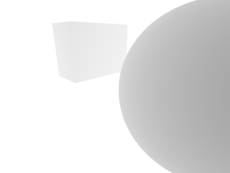
We once again get an Image from our pixel-buffer, but I also included a depth-buffer image with gray values (also as PPM). The darker the pixel color, the closer the object at that pixel is to the camera. As promised, I show the difference between perspective and orthogonal projection. I set the far plane of both types on the same size.

First perspective...

Perspective Pixel Buffer

Perspective Depth Buffer

...and orthogonal

Orthogonal Pixel Buffer

Orthogonal Depth Buffer

Conclusion

We discussed some transformation types for objects and that there are two different types of projections. To get a clue for colors we added a simple shader. We extended rasterization with depth queries and stored them in a depth buffer where we created an output image.

In the future we will hardly find usages for projection matrices. The only other case where they are needed is for Radiosity, but this is another story.

In the next issue we will go for Raycasting which can also be used for both orthogonal and perspective projection. But I think showing both won't be necessary. I also intend to only use perspective projection from now on, preparing both is not such an easy task. Also we will describe new shading models and upgrade the Material class.

Alright, see you in my next post.

Repository

https://github.com/rumpfc/CGG/tree/master/cgg04_3D_transform_viewing

Tested with:

• Visual Studio 2013 (Windows 8.1)
• GNU Compiler 4.9.2 (Ubuntu 12.04)